Megan Langford

SECTION I

Let’s begin by taking a look at the graph of a basic polar equation.

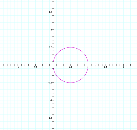
This appears to be a fairly complex equation to create such a simple graph. It appears as a circle with a radius of 0.5 that is centered at (0.5,0).

To see what effect k’s value has on the behavior of the equation, let’s modify our example by setting k=2 and keeping b set at b=1.

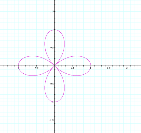
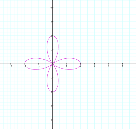
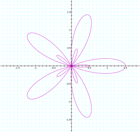
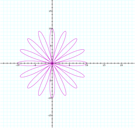
Surprisingly, our graph appears to take the shape of a flower with 4 petals. We can now hypothesize that the amount of petals for this equation is always equal to twice the k value. To test whether this is true, let’s set k=8 and keep our b value the same (1).

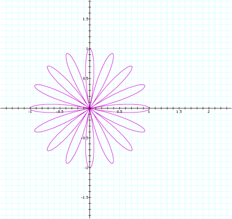
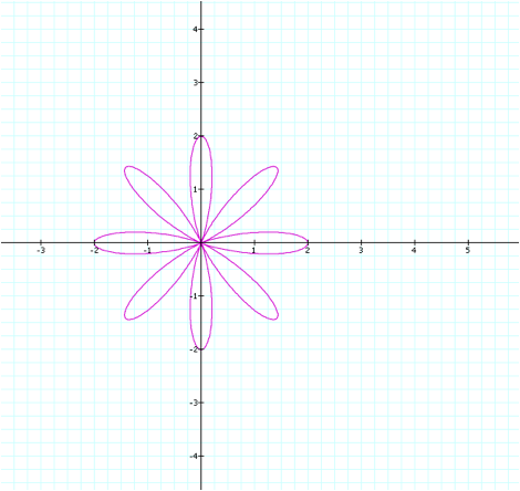
This is consistent with our hypothesis that the number of petals is twice the k value, since we have a total of 16 petals here and the k value is 8.

Another comparison we can make between the previous two graphs is that the petals extend between -1 and 1 on both the x and y axes. Could this behavior perhaps be correlated to the b value? Let’s examine the graph when the b value is increased. Here, b=3 and we will keep k=8.

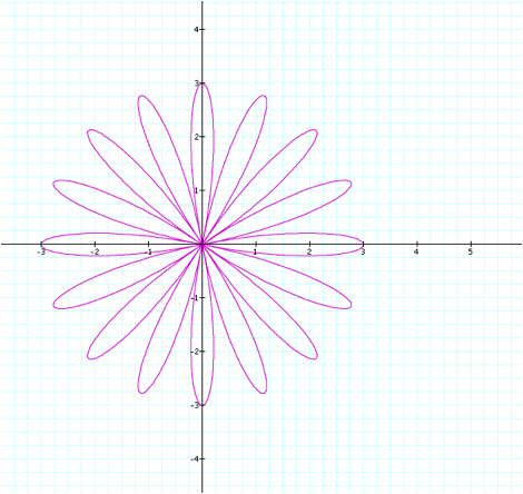
Not surprisingly, the number of petals has not changed, since we have not changed the k value. We can notice here that the petals appear to extend between -3 and 3 in all directions. Thus, our hypothesis does appear to be correct that the petals’ length is equal to the b value.

To verify this behavior, let’s test this hypothesis one more time as we set b=10 and keep k=8.

Again, this graph confirms our analysis is correct, since the petals extend between -10 and 10 along both axes when b=10.

Let’s take a step back and examine the case when our k value is an odd number. Will the same pattern hold true that we noticed for the even k values? We will test this by setting k=5 and keeping b=10.

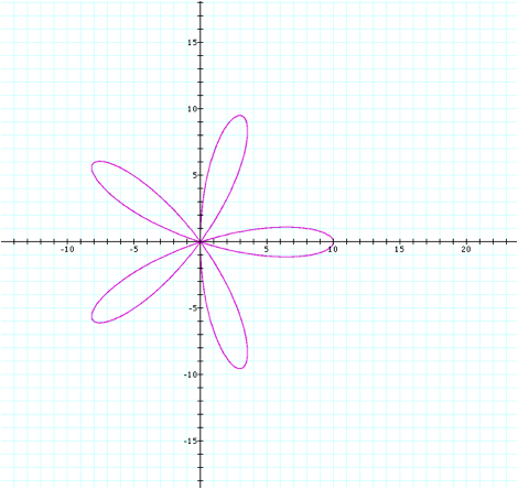
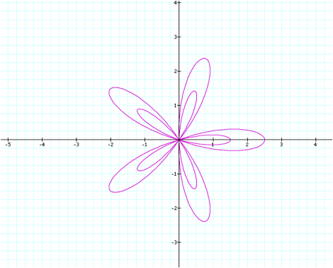
As a reminder, when k was an even number, we had a graph containing 2k petals. In this case, however, it appears that when k is an odd number, the graph contains k petals. For another look, we will graph with k=9 and b=10.

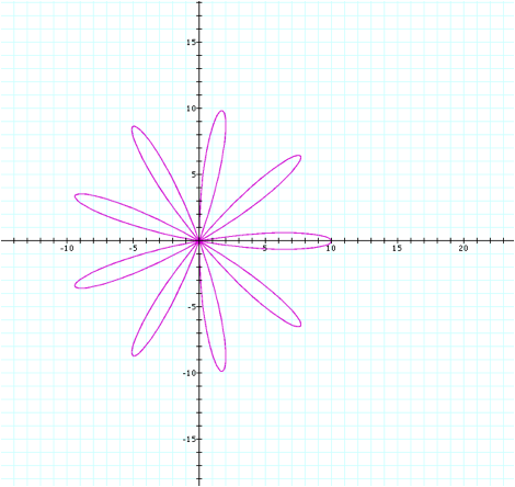
The odd number pattern is consistent in this graph, since k was set at 9, and there are 9 petals on the graph.

SECTION II

Now that we understand the basic behavior of the above function and its modifications, let’s take the function a step further and analyze the behavior of the graph when we consider also adding a term to the equation. Let’s call this the a term. To start with simplification, let’s set a=1, b=1, and k=1.

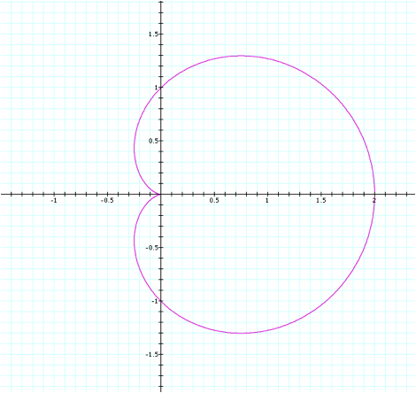
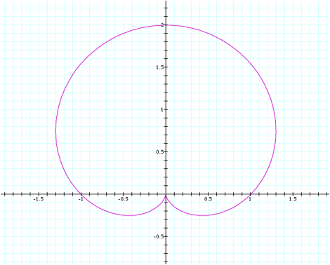
Recall that the first equation we graphed in this exercise ended up being a circle with a radius of 0.5 that was centered at (0.5,0). The only difference between the equation used to generate that graph and the equation used to generate this one is that added a term. There are several differences between the two graphs, although their shape is in part similar. The most immediate difference noticed is that there is an indention along the left-hand side of the circular figure in this graph. The indention comes in and “points” at the origin.

Additionally, ignoring the indention, we would notice that the circular figure this time has a “radius” of about 1.25 and is centered near (0.75,0).

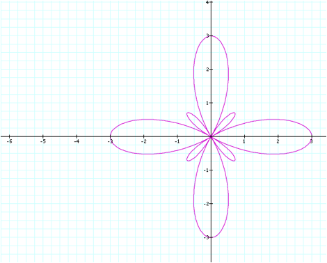
For comparison’s sake, let’s adjust the equation so that k=4. What changes will occur in the graph?

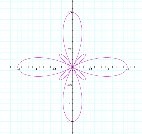
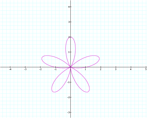
Curiously, the graph now appears more similar to some of the graphs we obtained in Part I. The first difference we can note, however, is that although we have set k to be an even number, the number of petals is equal to the k value (as opposed to twice the k value as in Part I).

Also, although our b value is set at 1, the petals have a length of 2. Let’s keep this in mind for later exploration. For now, let’s see if this pattern for the number of petals holds true if we increase the k value to another even number. Let’s test this by keeping a,b set at 1 and setting k=8.

Indeed, this hypothesis holds true in this case, since we have set k=8, and we have 8 petals on the figure. Well, we now understand the behavior when k is an even number, but what if k is an odd number? To explore this case, let’s leave a,b=1 and set k=5.

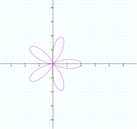
As it turns out, although the behavior of the graph in Part I changed when we changed k to be an odd number, the pattern in this case remains the same. Since we set k=5, there are 5 petals. This is consistent with what the graph was doing when k was an even number. To illustrate this one more time, let’s see the graph when we set k=9 (and leave a,b=1).

Again, the pattern holds because k=9 and there are 9 petals.

Now that we understand the impact of changing the k value, let’s explore what happens when we vary the value of the a term. Recall, when a=1, b=1, and k=4, we had the following graph:

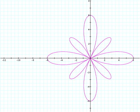
By comparison, let’s take a look at the graph when a=2, keeping all other terms the same.

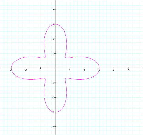
The most noticeable difference is that the petals no longer come together and meet at the origin in this graph. Instead, they form more of a cross shape, and the furthest point in towards the origin is about 0.75 away from each axis.

Another observation is that although we have kept b=1, the petals extend to -3 and 3 on each axis rather than coming to an end at -2 and 2 in the previous graph.

This does make sense because we are adding 2 to the equation we had previously, so logically we won’t be coming as close to the origin.

Let’s see if this trend continues as we increase the a value. On this next graph, let’s set a=7 and keep b and k the same.

The trend does appear to continue from the above graph. As we increased the a value, the petals became much less defined than they were in the prior example.

Additionally, the petals extend even further along the x and y axes, since they now reach all the way to positive and negative 8. These three examples all show a pattern that the petals each have a length of the a value plus one. In this case, since a=7, the petal length is 8.

In this manner, let’s continue to explore the case when . First, let’s set a=0.5 (where b=1 and k=4).

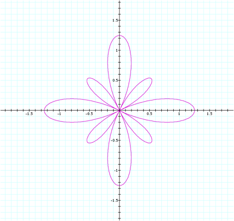
This is clearly not a shape that has been created by any other modification we have seen thus far. The larger flower’s petal length is 1.5, which is consistent with our pattern since 1.5=1+0.5 (and a=0.5). However, we now have a smaller petal shapes that appear in between each of the larger petals.

Let’s take a look when a takes on another decimal less than 1. Here, we graph when a=0.25, with all other values remaining the same.

The larger petals are still of the length a+1, since they appear to have length 1.25. The smaller petals have increased their length as well.

Now just to explore this new shape a bit further, let’s see if there is a difference in shape when k is set to be an odd number. Let’s keep a=0.25, change k to 5, and leave b=1 to view this scenario.

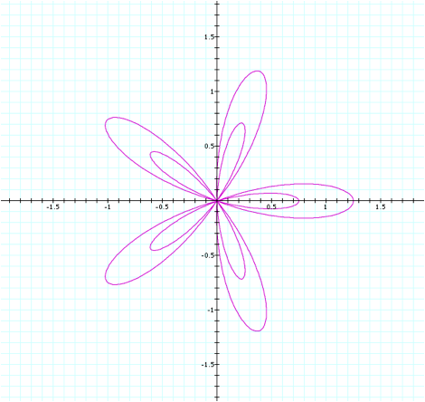
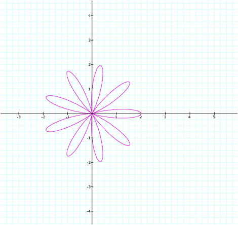
Surprisingly, it appears that if k is an odd number, the smaller flower shape actually appears inside of the larger one. The petal lengths all appear to remain unchanged in the scenario. Because we have changed the k value to 5, we now have 5 petals on each flower, which is consistent with the behavior we previously recognized.

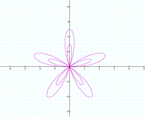
As a final exploration in this section, let’s set a back to 0.5 and keep b=1 and k=5 to see the difference in our most recent graph when the a value is slightly larger.

In this case, the petal length of the larger flower is as we would have expected, since 1+0.5=1.5. The smaller flower inside has actually decreased in size when we increased the a value. I would conjecture that since the smaller flower’s petal length was 0.75 when a=0.25 and 0.5 when a=0.5, then the length of the smaller flower’s petals is equal to 1-a.

Finally, let’s examine the effect a change in the b value has on the behavior of the graph. We will start by looking back at the graph we created with a=1, b=1, and k=4.

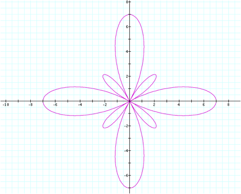
Now, let’s examine the change in the graph when we increase the b value. For this one, let’s set a=1, b=2, and k=4.

Notice that this graph is very similar in shape to the graph we had created when we set a=0.5, b=1, and k=4. The difference is that instead of the petals having a length of 1.5, the petal length is now 3 for the larger flower. The smaller flower also appears to have longer petals in this instance. In this case, the petals of the larger flower have a length of the b value plus one. To see if this pattern continues, we can test it again by graphing the equation using a=1, b=5, and k=4.

Again, this behavior is consistent because the b value is 5, and the petal length is 6. So throughout this section, we have hypothesized that the petal lengths are related to the a value plus one or the b value plus one. Which one is correct?

Well, actually they are both correct in the cases we were using. Notice that in each of these cases, the other value was set equal to 1. Meaning that if we were basing the petal length on the a value plus one, the b value was actually being set =1 (and vise versa). So in actuality, the length of the petals is a+b. To show this is the case, let’s create a graph where both a and b are greater than 1. Here, let a=2, b=5, and k=4.

In fact, our analysis is correct. Here, a+b = 2+5 = 7, and 7 is our petal length. The same is true for the petal length of our smaller flower. The length of the smaller flower is only 1-a when b=1. In general, the smaller flower’s petal length is b-a. To illustrate this point, let us take a look at the graph when a=0.5, b=2, and k=5.

Here, b-a = 2-0.5 = 1.5, and 1.5 is the smaller flower’s petal length.

To finalize our conjectures, we have determined that the petals will extend to the length of a+b and there will be k number of petals. We also know that if a is less than 1 or if b is larger than a, we will have a small flower as well as the original larger one. The length of the smaller flower’s petals is b-a. Also, if a is larger than b, the petals will not meet together at the origin.

SECTION III

We have now conducted an in-depth analysis of several modifications to the polar equation that includes the cosine function. Naturally, our next question would be whether or not this behavior remains the same when we are examining the case of the polar equation that includes the sine function.

Let’s first take a look at the instance where a, b, and k are all 1 and we are instead using the sine function in the graph.

This is very similar to the first graph from section 2 when we looked at the equation using the cosine function. It simply appears to have been rotated by 90 degrees. Let’s continue to change the values to see how similar the patterns remain. Here, let’s keep a and b set to 1, and let’s set k=4.

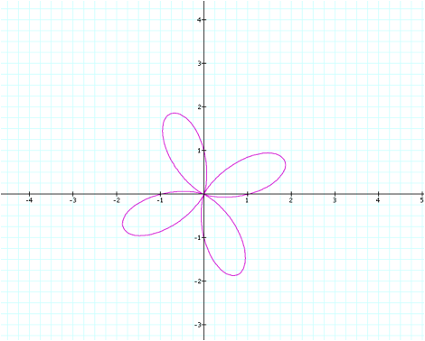
Here, the flower shape remains to be the same as the one created with similar values plugged into the cosine function. However, it does appear to have been rotated approximately 30 degrees.

To further examine this pattern, let’s adjust the k value to 5, keeping the a and b values the same.

The shape again is identical to the one with similar values plugged in to the cosine function, but again there appears to be some sort of rotation (although this time it appears to be possibly less than 30 degrees). I will let you continue to analyze this rotational behavior as a further exercise. For our purposes, let’s just take a look at the patterns we noticed in the last section and see if they still exist.

So far, there are still k number of petals, since we had 4 petals when k was 4 and 5 petals when k was 5. Since we have kept the a and b values at 1, the petal lengths in both graphs do indeed to appear to have a length a+b = 2.

Let’s try the case when a=0.5, b=2, and k=5. In our last problem, this meant that there would be a smaller flower inside of the larger one. Also, the smaller petals would have a length of b-a = 2-0.5 = 1.5, and the larger petals would have a length of a+b = 2+0.5 = 2.5. Will this be the case in this example as well?

Yes, this pattern holds for our sine function as well. The only difference is again, the rotation. We can continue to try different values for each of the variables, and we will continue to view the same patterns in the sine function, with the only difference being a rotation of some sort. In this manner, these basic behaviors remain the same for both sine and cosine polar equations.